相关性分析及散点图绘制-脚本使用
相关性分析是指对两个或多个具备相关性的变量进行分析,从而衡量变量间的相关程度。变量之间相关程度的量化使用相关系数r,常见的相关系数有Pearson相关系数、Spearman相关系数以及Kendall相关系数。相关性散点图可以更直观清晰地展现相关性分析的结果,常用于生信分析中。
例如:在一篇2021年发表于Briefings in Bioinformatics上的影响因子为11.62的文献中,作者大量地进行相关性分析并绘制了散点图,更好地展示了相关性分析的结果。
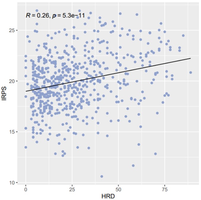
下图是文献中免疫相关预后评分(IRPS)与一些决定肿瘤免疫原性的潜在因素(如突变负荷、同源重组缺陷等)的相关性散点图,并且作者在图中还添加了相关系数r、显著性p值以及拟合曲线,从中可以直观地看出IRPS与这些因素中的大部分都有显著的负相关关系。

为了使大家能更简便快捷地绘制出精美的相关性散点图,这里我们给大家提供一个绘制相关性散点图的R脚本,这个脚本只需要准备好相应的输入文件,再进行简单的命令行操作即可在两个变量间进行相关性分析并绘制出散点图。
使用命令示例如下
Rscript /share/work/fangs/scripts/tcga/cor_scatter_plot.r -m metadata_all.tsv \
    -n IRPS -c HRD -t pearson -H 5 -W 5 -o corrplot -p IRPS_HRD
输入文件准备
这个脚本所必需的输入文件只有一个,通过-m参数指定(metadata_all.tsv),文件中每一行为一个样本,列必须包含要进行相关性分析的两个变量,且两个变量需为数值型数据,如下列表格所示:
| barcode | HRD | IRPS |
| TCGA-A1-A0SB-01A-11R-A144-07 | 0 | 13.47 |
| TCGA-A1-A0SD-01A-11R-A115-07 | 25 | 20.22 |
| TCGA-A1-A0SE-01A-11R-A084-07 | 15 | 19.54 |
更多脚本参数设置及说明
初次使用脚本时,可以通过-h参数获得以下帮助信息。
Rscript cor_scatter_plot.r -h
usage: cor_scatter_plot.r [-h] -m meta [-n name] [-c cor_name] [--log2]
                          [-t method] [-l color] [-s size] [-H HEIGHT]
                          [-W WIDTH] [-o OUTDIR] [-p PREFIX]

Correlation scatter plot

optional arguments:
  -h, --help            show this help message and exit
  -m meta, --meta meta  Input contains two columns of data for calculating the
                        correlation[required]
  -n name, --name name  Specifies the column name of the
                        column[optional,default:IRPS]
  -c cor_name, --cor_name cor_name
                        The column name that computes correlation with the
                        specified column[optional,default:PDCD1]
  --log2                Whether to perform log2
                        processing[optional,default:False]
  -t method, --method method
                        Specifies the method to calculate the correlation[opti
                        onal:pearson/Spearman/...,default:pearson]
  -l color, --color color
                        Specifies the color of the fitting
                        curve[optional,default:black]
  -s size, --size size  Specify the thickness of the fitting
                        curve[optional,default:0.5]
  -H HEIGHT, --height HEIGHT
                        the height of dumbbell plot[optional,default 8]
  -W WIDTH, --width WIDTH
                        the width of dumbbell plot[optional,default 8]
  -o OUTDIR, --outdir OUTDIR
                        output file directory[optional,default cwd]
  -p PREFIX, --prefix PREFIX
                        out file name prefix[optional,default kegg]
根据自身需要调整必要的参数:
-n 输入列名,指定进行相关性分析的其中一个变量(y轴);
-c 输入列名,指定进行相关性分析的另一个变量(x轴);
-t 指定相关性分析的方法,如pearson、Spearman等;
-l 指定拟合曲线的颜色,默认为黑色;-s 指定拟合曲线的粗细,默认为0.5。
其他参数说明
--log2 加上该参数即要对连续变量进行log2转化;
-H 指定输出图片的高度,默认高为6英寸;
-W 指定输出图片的宽度,默认宽为8英寸;
-o 指定结果输出的路径,默认为当前路径;
-p 指定输出文件名字的前缀。
脚本获取方法
在”生信博士“公众号回复cor_scatter_plot即可获得网盘链接以及提取码。
如何使用命令行的方法分析数据
可能有的人没有用过命令的形式分析数据, 可以学习下面的课程入门一下:

- 发表于 2022-06-10 14:29
- 阅读 ( 8191 )
- 分类:R
