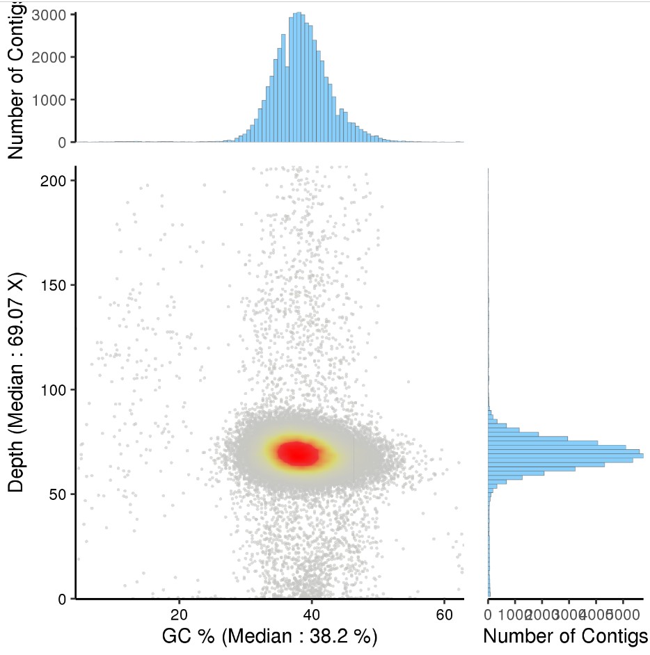
基因组组装GC 含量与深度图:
基因组组装GC 含量与深度图:
library("argparse")
############################################################################
#北京组学生物科技有限公司
#author huangls
#date 2022.07.10
#version 1.0
#学习R课程:
#R 语言入门与基础绘图:
# https://zzw.h5.xeknow.com/s/2G8tHr
#R 语言绘图ggplot等等:
# https://zzw.h5.xeknow.com/s/26edpc
###############################################################################################

parser <- ArgumentParser(description='Seurat single cell DimPlot analysis :https://satijalab.org/seurat/reference/dimplot')
parser$add_argument( "-i", "--gc.table", type="character",required=T, default=NULL,
help="input single Seurat obj in rds file [required]",
metavar="filepath")
parser$add_argument( "-d", "--depth.table", type="character",required=T, default=NULL,
help="input single Seurat obj in rds file [required]",
metavar="filepath")
parser$add_argument( "--mingc", type="double",required=F, default=0,
help="min gc cut  [default  %(default)s]",
metavar="mingc")
parser$add_argument( "--maxgc", type="double",required=F, default=1,
help="min gc cut  [default  %(default)s]",
metavar="maxgc")
parser$add_argument( "--mindp", type="integer",required=F, default=0,
help="min depth cut  [default  %(default)s]",
metavar="mindepth")
parser$add_argument( "--maxdp", type="integer",required=F, default=500,
help="min depth cut  [default  %(default)s]",
metavar="maxdepth")


parser$add_argument( "--pt.size ", type="double", default=0.7,
help="Adjust point size for plotting [default  %(default)s]",
metavar="pt.size")
parser$add_argument( "-H", "--height", type="double", default=5,
help="the height of pic   inches  [default  %(default)s]",
metavar="height")
parser$add_argument("-W", "--width", type="double", default=5,
help="the width of pic   inches [default  %(default)s]",
metavar="width")
parser$add_argument( "-o", "--outdir", type="character", default=getwd(),
help="output file directory [default  %(default)s]",
metavar="path")
parser$add_argument("-p", "--prefix", type="character", default="demo",
help="out file name prefix [default  %(default)s]",
metavar="prefix")
opt <- parser$parse_args()
#####################################################

if( !file.exists(opt$outdir) ){
if( !dir.create(opt$outdir, showWarnings = FALSE, recursive = TRUE) ){
stop(paste("dir.create failed: outdir=",opt$outdir,sep=""))
}
}

##################
library(ggplot2)
library(tibble)
library(dplyr)
library(aplot)
gc <- read.table(opt$gc.table, header = F , row.names = 1)
dp <- read.table(opt$depth.table, header = F , row.names = 1 )
gc1 <- rownames_to_column(gc,var = "id")
dp1 <- rownames_to_column(dp,var = "id")
gcdep <- inner_join(gc1, dp1, by = "id")
colnames(gcdep) <- c("id", "GC", "Depth")
#p <- ggplot( data = gcdep )  +
#geom_point(aes(x=GC,y=Depth),pch=16, colour = "red", alpha = 0.5 ,cex = opt$pt.size) +
#xlab("GC content")  +
#ylab("Depth") +
#xlim(opt$mingc, opt$maxgc) +
#ylim(opt$mindp, opt$maxdp) +
#theme_bw()+theme(
#panel.grid=element_blank(),
#axis.text.x=element_text(colour="black"),
#axis.text.y=element_text(colour="black"),
#panel.border=element_rect(colour = "black"),
#legend.key = element_blank(),
#legend.title = element_blank())


library(grid)
gcdep=as.data.frame(gcdep)
head(gcdep)
#GC 含量中位数(百分比)
gcdep$GC <- 100 * gcdep$GC
GC_median <-  round(median(gcdep$GC), 2)
#测序深度中位数
depth_median <- round(median(gcdep$Depth), 2)
#为了避免二代测序的 duplication 所致的深度极高值,将高于测序深度中位数 3 倍的数值去除
gcdep <- subset(gcdep, Depth <= 3 * depth_median)

#depth 深度、GC 含量散点密度图
gc <- ggplot(gcdep, aes(GC, Depth)) +
geom_point(color = 'gray', alpha = 0.6, pch = 16, size = 0.5) +
#geom_vline(xintercept = GC_median, color = 'red', lty = 2, lwd = 0.5) +
#geom_hline(yintercept = depth_median, color = 'red', lty = 2, lwd = 0.5) +
stat_density_2d(aes(fill = ..density.., alpha = ..density..), geom = 'tile', contour = FALSE, n = 500) +
scale_fill_gradientn(colors = c('transparent', 'yellow', 'red', 'red')) +
labs(x = paste('GC % (Median :', GC_median, '%)'), y = paste('Depth (Median :', depth_median, 'X)')) +
theme_bw()+theme(
panel.grid=element_blank(),
axis.text.x=element_text(colour="black"),
axis.text.y=element_text(colour="black"),
#panel.border=element_rect(colour = "black"),
legend.key = element_blank(),
panel.border= element_blank(),
legend.position = 'none',
#axis.ticks.length = unit(0, "pt"),
plot.margin = margin(t = 0,  # Top margin
r = 0,  # Right margin
b = 0,  # Bottom margin
l = 20), # Left margin
axis.line.y.left=element_line(colour = "black"),
axis.line.y.right=element_blank(),
axis.line.x.top = element_blank(),
axis.line.x.bottom = element_line(colour = "black"),
legend.title = element_blank())+coord_cartesian(expand = FALSE)
#depth 深度频数直方图
depth_hist <- ggplot(gcdep, aes(Depth)) +
geom_histogram(binwidth = (max(gcdep$Depth) - min(gcdep$Depth))/100, fill = 'LightSkyBlue', color = 'gray40', size = 0.1) +
labs(x = '', y = 'Number of Contigs') +
coord_flip(expand = FALSE) +
#geom_vline(xintercept = depth_median, color = 'red', lty = 2, lwd = 0.5)+
theme_bw()+theme(
panel.grid=element_blank(),
#axis.text.x=element_blank(),
#axis.text.y=element_text(colour="black"),
#panel.border=element_rect(colour = "black"),
panel.border= element_blank(),
legend.key = element_blank(),
axis.text.y=element_blank(),
axis.ticks.y=element_blank(),
panel.spacing = unit(0, "cm"),
axis.ticks.length.y = unit(0, "pt"),
plot.margin = margin(t = 0,  # Top margin
r = 0,  # Right margin
b = 0,  # Bottom margin
l = 0), # Left margin
axis.line.y.left=element_blank(),
axis.line.y.right=element_blank(),
axis.line.x.top = element_blank(),
axis.line.x.bottom = element_line(colour = "black"),
legend.title = element_blank())
#GC 含量频数直方图
GC_hist <- ggplot(gcdep, aes(GC)) +
geom_histogram(binwidth = (max(gcdep$GC) - min(gcdep$GC))/100, fill = 'LightSkyBlue', color = 'gray40', size = 0.1) +
labs(x = '', y = 'Number of Contigs') +
#geom_vline(xintercept = GC_median, color = 'red', lty = 2, lwd = 0.5)+
theme_bw()+theme(
panel.grid=element_blank(),
#axis.text.x=element_text(colour="black"),
#axis.text.y=element_text(colour="black"),
#panel.border=element_rect(colour = "black"),
panel.border= element_blank(),
legend.key = element_blank(),
axis.text.x=element_blank(),
axis.ticks.x=element_blank(),
panel.spacing = unit(0, "cm"),
axis.ticks.length.x = unit(0, "pt"),
plot.margin = margin(t = 0,  # Top margin
r = 0,  # Right margin
b = 0,  # Bottom margin
l = 20), # Left margin
axis.line.x.top=element_blank(),
axis.line.x.bottom = element_blank(),
axis.line.y.right= element_blank(),
axis.line.y.left = element_line(colour = "black"),
legend.title = element_blank())+coord_cartesian(expand = FALSE)


png(filename=paste(opt$outdir,"/",opt$prefix,".png",sep=""), height=opt$height*300, width=opt$width*300, res=300, units="px")
grid.newpage()
# pushViewport(viewport(layout = grid.layout(3, 3)))
# print(gc, vp = viewport(layout.pos.row = 2:3, layout.pos.col = 1:2))
# print(GC_hist, vp = viewport(layout.pos.row = 1, layout.pos.col = 1:2))
# print(depth_hist, vp = viewport(layout.pos.row = 2:3, layout.pos.col = 3))
#
p <- gc %>%
 insert_top(GC_hist, height=.3) %>%
 insert_right(depth_hist, width=.4)
p
dev.off()


pdf(file=paste(opt$outdir,"/",opt$prefix,".pdf",sep=""), height=opt$height, width=opt$width)
p <- gc %>%
  insert_top(GC_hist, height=.3) %>%
  insert_right(depth_hist, width=.4)
p
dev.off()
- 发表于 2022-07-08 19:58
- 阅读 ( 4606 )
- 分类:R